Support Vector Machine Learning

Project Details

Data Description

Iris flower classification is a popular dataset in machine learning project. The dataset contains three classes of flowers: Versicolor, Virginica, Setosa and each class has 4 features like “Sepal length”, “Sepal width”, “Petal length” and “ Petal width”. The goal of the iris flower classification is to train the SVM mode and predict flowers based on their features.

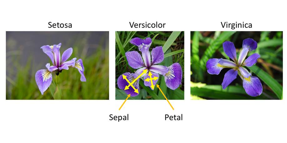
As the dataset have labeled the variable, it is supervised machine learning. Supervised machine learning are types of machine learning that are trained on well-labeled training data. Labeled data means that training data is already tagged with correct output.

In this project, I will solve the problem using the algorithm: Support vector machine as it is a supervised machine learning algorithm which analyzes data for classification and regression. Also, SVMSs are one of the most robust classification methods.

How SVM works?

SVM approximates a line (hyperplane) separating data between two classes.

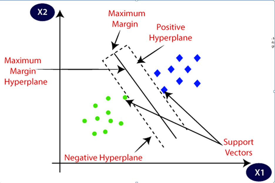
SVM algorithm finds the points closest to the line form two classes. These points are known as support vectors. Then, it computes the distance between the line and support vectors. The distance is called margin. The main purpose is to maximize the margin. The hyperplane which has maximum margin is known as the optimal hyperplane.

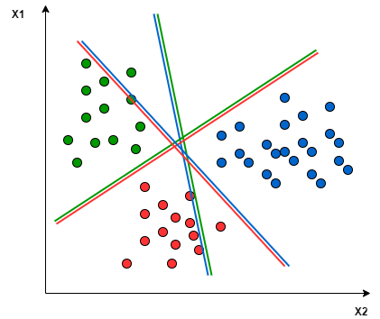
It mainly supports binary classification natively. For multiclass classification, it separates the data for binary classification and uses the same method repeatedly to break down multi-classification problems into multiple binary classification problems.

Python Packages:

1. Numpy
2. Matplotlib
3. Seaborn
4. Pandas
5. Scikit-learn

Roadmap:

1. Load the data
2. Analyze and visualize the dataset
3. Split a dataset into training and testing datasets
4. Train the model
5. Model Evaluation
6. Testing the model

Step 1:

Import packages:

#import libaries 
import numpy as np
import matplotlib.pyplot as plt
import seaborn as sns
import pandas as pd
from sklearn.model_selection import train_test_split
from sklearn.svm import SVC
from sklearn.metrics import accuracy_score
from sklearn.metrics import classification_report
		    

First, I imported necessary packages for this project.

Pandas will used to load data from various sources like local or cloud storage, database, excel file, CSV file and so on.

Numpy will be used for any computational operations.

Matplotlib and seaboarn will be used for data visualization.

csv_url = 'url'
columns = ['Sepal length', 'Sepal width', 'Petal length', 'Petal width', 'Class_labels']
# Load the data
df = pd.read_csv(csv_url, names=columns)
# display first 5 rows data
print(df.head())
		    

As I use the data from web server, I define the url variable and then use read_csv to read data and set the column name as per the iris data information.

Look at first the five-row data in the dataset.

Step2: Analyze and visualize the dataset.

# display base statistical analysis regarding the data
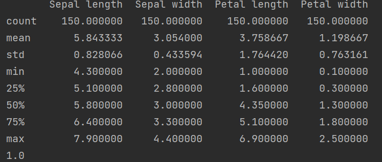
print(df.describe())
		    

From this data description, I can see all the data descriptions on the data, like mean length and width in Sepal and Petal, min and max values and 25%, 50% and 75% distribution values.

Let’s visualize the dataset.

Seaborn pair plot method helps visualize the whole dataset.

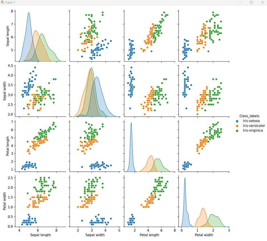
# visualize the dataset by labeled variable
sns.pairplot(df, hue='Class_labels')
plt.show()
		    

By looking the visualization, it is very clear that virginica is well-separated from setosa and versicolor.

Virginica is longest flower and setosa is the shortest.

# Separate features and target
data = df.values
X = data[:,0:4]
Y = data[:,4]
		    

X is featuring dataset including all variable used to train the model.

Y is labeled dataset including target values.

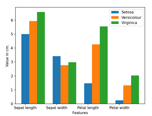
# Calculate average of each features for all classes
Y_Data = np.array([np.average(X[:, i][Y==j].astype('float32')) for i in range (X.shape[1])
 for j in (np.unique(Y))])
Y_Data_reshaped = Y_Data.reshape(4, 3)
Y_Data_reshaped = np.swapaxes(Y_Data_reshaped, 0, 1)
X_axis = np.arange(len(columns)-1)
width = 0.25
		    

Calculates the average from ab array.

I used two for loops inside a list. This is known as list comprehension.

List comprehension helps reduce number of lines of code.

The Y_Data is the 1 D array. But I have 4 features for every 3 classes. So I reshaped Y_Data to a (4,3) shaped array.

Then, I change the axis of the reshaped matrix.

# Plot the average
plt.bar(X_axis, Y_Data_reshaped[0], width, label = 'Setosa')
plt.bar(X_axis+width, Y_Data_reshaped[1], width, label = 'Versicolour')
plt.bar(X_axis+width*2, Y_Data_reshaped[2], width, label = 'Virginica')
plt.xticks(X_axis, columns[:4])
plt.xlabel("Features")
plt.ylabel("Value in cm.")
plt.legend(bbox_to_anchor=(1.3,1))
plt.show()
		    

I present data using matplotlib to show average in bar chart.

I can see the virginica is the longest and setosa is shortest clearly.

Step3: Split a dataset into training and testing datasets

X_train, X_test, y_train, y_test = train_test_split(X, Y, test_size=0.2)
		    

I split the whole dataset into two groups: training dataset and testing dataset using train_test_split by 80% verse 20%. I will use the testing dataset to check the accuracy of the mode later.

Step4: Train the model

# Prediction of classifier
svn = SVC()
svn.fit(X_train, y_train)
		    

Initialize support vector classifier class from scikit-learn package to svn variable.

I feed training dataset and labeled dataset into the algorithm using fit() method.

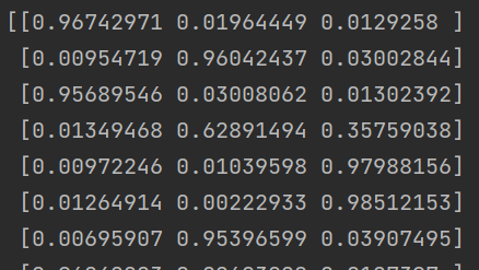
# Probability of each class
svn_prob = SVC(probability=True)
svn_prob.fit(X_train, y_train)
pred_prob=svn_prob.predict_proba(X_test)
		    

I also use same method and add a parameter to calculate probability for each class. Here I just add probability=True.

Above are results in array format: setosa, versicolor, virginica order. Basically, it takes largest probability as output result.

Step 5: Model Evaluation

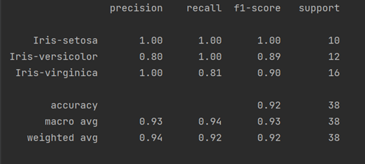
pred = svn.predict(X_test)
print("Accuracy Score:" + str(round(accuracy_score(y_test, pred),2)))
		    

I predicted the classes from testing dataset using my trained model.

Check the accuracy score of the predicted results.

Accuracy_score takes true values and predicted values and return percentage of accuracy.

The accuracy is above 92%. Another interesting finding is when I allocate more data into training data, the accuracy is increased as well. It prove a saying: more data, better model, more accuracy.

I also show the detailed classification repot based the testing dataset.

print(classification_report(y_test, pred))
		    

The report indicates detailed information of the prediction.

Precision defines the ration of true positives to the sum of true positive and false positive.

Recall defines the ratio of true positive to sum of true positive and false negative.

F1-score is the mean of precision and recall results.

Support is the number of actual occurrences of the class in the testing dataset.

Accuracy is the average of f1-scores.

Step 6: Testing the Model

X_new = np.array([[3, 2, 1, 0.2], [4.9, 2.2, 3.8, 1.1], [5.3, 2.5, 4.6, 1.9]])
pred_new = svn.predict(X_new)
print("Prediction of Species: {}".format(pred_new))
		    

I just randomly generated values based on the average plot to see if the model work correctly.

It looks like the model predicts correctly because the outputs meet expectations that setosa is shortest and virginica is longest and versicolor is in the middle.

#Save the model
with open('SVM.pickle', 'wb') as f:
    pickle.dump(svn, f)
# Load the model
with open('SVM.pickle', 'rb') as f:
    model = pickle.load(f)
model.predict(X_new)
		    

I can save the model using pickle format.

I can load the trained model in any other program using pickle and use it to predict the iris data.