Classification Random Forest

Project Details

Description

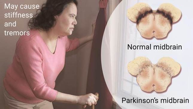
Parkinson's disease is a brain disorder that causes unintended or uncontrollable movements, such as shaking, stiffness, and difficulty with balance and coordination. Symptoms usually begin gradually and worsen over time. As the disease progresses, people may have difficulty walking and talking. The dataset contains two classes of status: 1 meaning yes and 0 meaning no and each class has 24 features.

Data Description:

name - ASCII subject name and recording number

MDVP:Fo(Hz) - Average vocal fundamental frequency

MDVP:Fhi(Hz) - Maximum vocal fundamental frequency

MDVP:Flo(Hz) - Minimum vocal fundamental frequency

MDVP:Jitter(%),MDVP:Jitter(Abs),MDVP:RAP,MDVP:PPQ,Jitter:DDP - Several

measures of variation in fundamental frequency

MDVP:Shimmer,MDVP:Shimmer(dB),Shimmer:APQ3,Shimmer:APQ5,MDVP:APQ,Shimmer:DDA - Several measures of variation in amplitude

NHR,HNR - Two measures of ratio of noise to tonal components in the voice

status - Health status of the subject (one) - Parkinson's, (zero) - healthy

RPDE,D2 - Two nonlinear dynamical complexity measures

DFA - Signal fractal scaling exponent

spread1,spread2,PPE - Three nonlinear measures of fundamental frequency variation

The goal of the Parkinson’s disease is to train the random forest model, analyze importance of variables, tuning the accuracy of model, predict status based on their features.

As the dataset have labeled the variable, it is supervised machine learning. Supervised machine learning are types of machine learning that are trained on well-labeled training data. Labeled data means that training data is already tagged with correct output.

In this project, I will solve the problem using the algorithm: Random Forest as it is a supervised machine learning algorithm which analyzes data for classification and regression. Also, Random Forest Classification is one of the most robust classification methods.

How Random Forest Algorithms work?

Random forest algorithms have three main hyperparameters, which need to be set before training. These include node size, the number of trees, and the number of features sampled. From there, the random forest classifier can be used to solve for regression or classification problems.

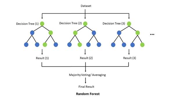
The random forest algorithm is made up of a collection of decision trees, and each tree in the ensemble is comprised of a data sample drawn from a training set with replacement, called the bootstrap sample. Of that training sample, one-third of it is set aside as test data, known as the out-of-bag (oob) sample, which we’ll come back to later. Another instance of randomness is then injected through feature bagging, adding more diversity to the dataset and reducing the correlation among decision trees. Depending on the type of problem, the determination of the prediction will vary. For a regression task, the individual decision trees will be averaged, and for a classification task, a majority vote—i.e. the most frequent categorical variable—will yield the predicted class. Finally, the oob sample is then used for cross-validation, finalizing that prediction.

Python Packages:

1. Matplotlib

2. Seaborn

3. Pandas

4. Scikit-learn

Roadmap:

1. Load the data

2. Analyze and visualize the dataset

3. Split a dataset into training and testing datasets

4. Train the model

5. Model Evaluation

6. Testing the model

7. Improving performance

Step 1:

Import packages:

#import libaries
import pandas as pd
import seaborn as sns
import numpy as np
from sklearn.model_selection import train_test_split
from sklearn.metrics import accuracy_score
from sklearn.ensemble import RandomForestClassifier
from sklearn.ensemble import BaggingClassifier
import matplotlib.pyplot as plt
from sklearn.metrics import classification_report
		    

First, I imported necessary packages for this project.

Pandas will used to load data from various sources like local or cloud storage, database, excel file, CSV file and so on.

Matplotlib and seaboarn will be used for data visualization.

Sklearn will be used for data split, accuracy report and modeling.

url=r'url'
df=pd.read_csv(url)
print(df.head())
		    

As I use the data from web server, I define the url variable and then use read_csv to read data and set the column name as per the Parkinsons data information.

Look at the first five-row data in the dataset.

Step 2: Analyze and visualize the dataset

# display base statistical analysis regarding the data
print(df.describe())
		    

From this data description, I can see all the data descriptions on the data, like mean in different measurements, min and max values and 25%, 50% and 75% distribution values.

Let’s visualize the dataset.

Seaborn pair plot method helps visualize the whole dataset.

# visualize the dataset by labeled variable
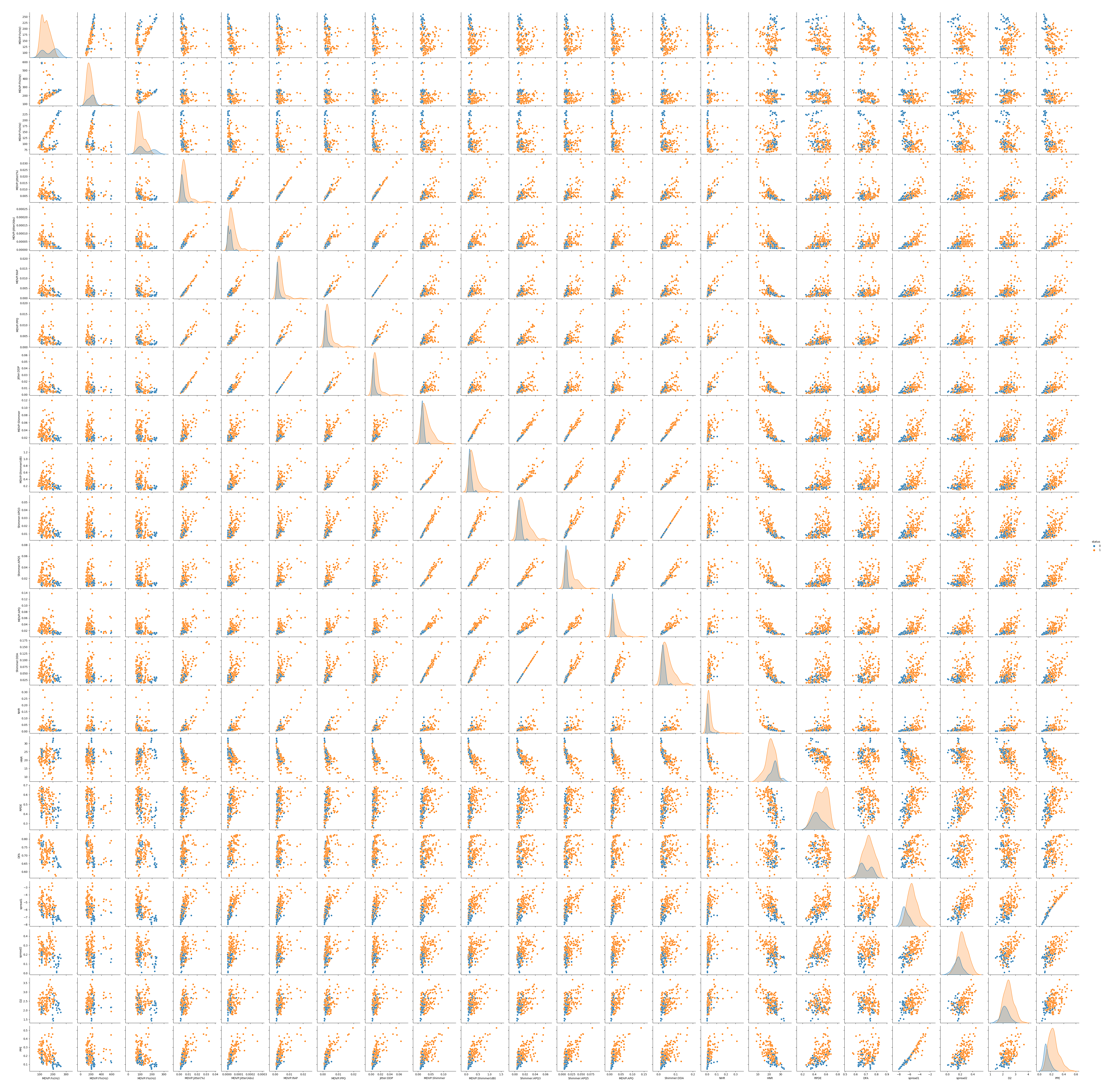
sns.pairplot(df, hue='status')
plt.savefig('parkinsons variable analysis')
		    

By looking the visualization, it is very clear that those whose status is yes have all values higher than those whose status is no.

# Separate features and target
X=df.loc[:,df.columns!='status'].values[:,1:]
Y=df.loc[:,'status'].values
feature=df.drop('status', axis=1)
feature_list=list(feature.columns)
Y = data[:,4]
		    

X is featuring dataset including all variable used to train the model.

Y is labeled dataset including target values.

Step3: Split a dataset into training and testing datasets

# Split the dataset
X_train,X_test,y_train,y_test=train_test_split(X, Y, test_size=0.2, random_state=42)
		    

I split the whole dataset into two groups: training dataset and testing dataset using train_test_split by 80% verse 20%. I will use the testing dataset to check the accuracy of the mode later.

Step3: Train the model

X_train, X_test, y_train, y_test = train_test_split(X, Y, test_size=0.20, random_state=42)
		    

I split the whole dataset into two groups: training dataset and testing dataset using train_test_split by 80% verse 20%. I will use testing dataset to check the accuracy of the mode later.

Step 4: Train the model

model=RandomForestClassifier(n_estimators=10,random_state=42)
model.fit(X_train,y_train)
		    

Initialize random forest classifier class from scikit-learn package to model variable.

Set the number of estimators as 10 which can be tuned to improve accuracy. Later I will talk about how to use elbow method.

I feed training dataset and labeled dataset into the algorithm using fit() method.

Step 5: Model Evaluation

pred=model.predict(X_test)
print('First Run Performance:'+str(accuracy_score(y_test,pred)*100))
		    

I predict the classes from testing dataset using my trained model.

Check the accuracy score of the predicted results.

Accuracy_score takes true values and predicted values and return percentage of accuracy.

The accuracy is above 92%.

I also show the detailed classification report based the testing dataset.

The report indicates detailed information of the prediction.

Precision defines the ration of true positives to the sum of true positive and false positive.

Recall defines the ratio of true positive to sum of true positive and false negative.

F1-score is the mean of precision and recall results.

Support is the number of actual occurrences of the class in the testing dataset.

Accuracy is the average of f1-scores.

Step 6: Testing the Model

#Testing the model
X_new = np.array([[114.38000,130.10900,104.63400,0.00332,0.00003,0.00160,0.00199,0.00480,0.01503,0.13700,0.00812,0.00933,0.01133,0.02436,0.00401,26.00500,0.405991,0.761255,-5.966779,0.197938,1.974857,0.184067],
                  [117.38800,125.03800,110.97000,0.00346,0.00003,0.00169,0.00213,0.00507,0.01725,0.15500,0.00874,0.01021,0.01331,0.02623,0.00415,26.14300,0.361232,0.763242,-6.016891,0.109256,2.004719,0.174429],
                  [151.73700,190.20400,129.85900,0.00314,0.00002,0.00135,0.00152,0.00506,0.01469,0.13200,0.00728,0.00886,0.01230,0.02184,0.00570,24.15100,0.396610,0.745957,-6.486822,0.197919,2.449763,0.132703]])
pred_new = model.predict(X_new)
# expected results:0,0,1
print("Prediction of Species: {}".format(pred_new))
		    

I just randomly generated values based on the average plot to see if the model work correctly.

It looks like the model predicts correctly because the outputs meet expectations that several key features have much higher values than others.

Step 7: Improving Performance

# bagging estimate
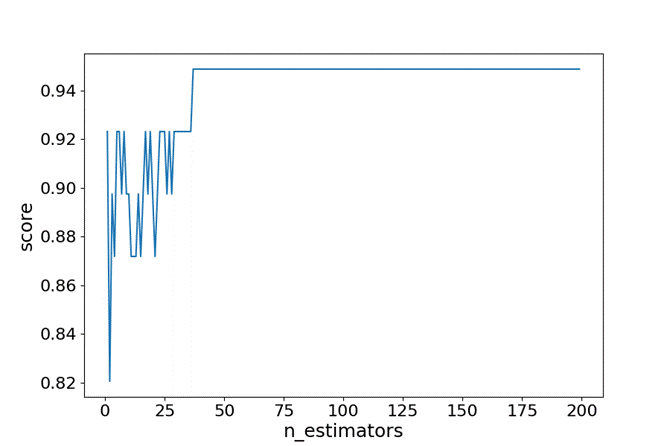
estimator_range = [e for e in range(1,200)]
models = []
scores = []

for n_estimators in estimator_range:

    # Create bagging classifier
    clf = BaggingClassifier(n_estimators = n_estimators, random_state = 42)

    # Fit the model
    clf.fit(X_train,y_train)

    # Append the model and score to their respective list
    models.append(clf)
    scores.append(accuracy_score(y_true = y_test, y_pred = clf.predict(X_test)))

# Generate the plot of scores against number of estimators
plt.figure(figsize=(9,6))
plt.plot(estimator_range, scores)

# Adjust labels and font (to make visable)
plt.xlabel("n_estimators", fontsize = 18)
plt.ylabel("score", fontsize = 18)
plt.tick_params(labelsize = 16)

# Visualize plot
# plt.show()
plt.savefig('bagging estimation')
		    

I used hyperparameter tuning. This is a complicated phrase that means “adjust the setting to improve the performance” (The setting are known as hyperparameters to differentiate them from model parameters learned during the training). In this example above, I used grid search method to get better performance.

• Define the range from 1 to 200.
• Use bagging classifier to try one by one and log the result for later analysis.
• Plot the graph to assess the result and save it as output.

To quantify the usefulness of all the variables in the whole random forest, I can look at the relative importance of the variables. The returned importance in the package indicates how much including a specific variable improves the prediction. I can use the numbers to make relative comparison among variables.

The top 5 are MDVP:Fo(Hz) - Average vocal fundamental frequency, PPE: nonlinear measures of fundamental frequency variation, spread1: nonlinear measures of fundamental frequency variation, MDVP:Fhi(Hz) - Maximum vocal fundamental frequency, MDVP:Flo(Hz) - Minimum vocal fundamental frequency and MDVP:Jitter(Abs): the measures of variation in fundamental frequency. It tells me these play more important role than others in predicting status of Parkinsons.

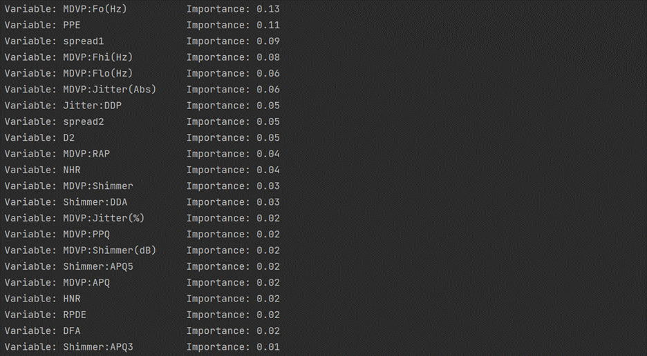
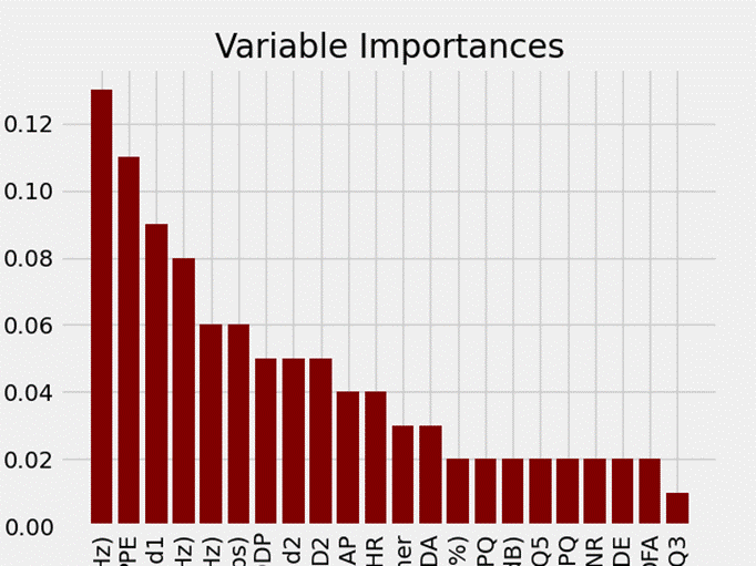
# Visualizations
# Make a bar chart
name=[]
value=[]

for pair in feature_importances:
    name.append(pair[0])
    value.append(pair[1])

plt.style.use('fivethirtyeight')
plt.bar(name, value, color='maroon', orientation = 'vertical')
# Tick labels for x axis
plt.xticks(rotation='vertical')
# Axis labels and title
plt.ylabel('Importance'); plt.xlabel('Variable'); plt.title('Variable Importances');
plt.show()
		    

I also visualized the importance of these variables to have clear understanding.

# Performence Improvement
# New random forest with only the two most important variables
rf_most_important = RandomForestClassifier(n_estimators=30,random_state=42)
# Extract the two most important features
important_indices=[feature_list.index('MDVP:Fo(Hz)'),feature_list.index('PPE'),feature_list.index('spread1'),feature_list.index('MDVP:Fhi(Hz)'),feature_list.index('MDVP:Flo(Hz)')
                  ,feature_list.index('MDVP:Jitter(Abs)'),feature_list.index('Jitter:DDP'),feature_list.index('spread2'),feature_list.index('D2')]
X_train_important=X_train[:,important_indices]
X_test_important=X_test[:,important_indices]
# Train the random forest
rf_most_important.fit(X_train_important,y_train)
# Make predictions and determine the error
predictions=rf_most_important.predict(X_test_important)
print('Performence Improvement:'+str(accuracy_score(y_test,predictions)*100))
print(classification_report(y_test, pred))		
			

Based on findings on importance of variables and, I dropped some variables for performance improvement and re-ran the model and tested results. They are same but sometimes accuracy may be infected by dropping some variables.