Multi-class Classification

Project Details

Description

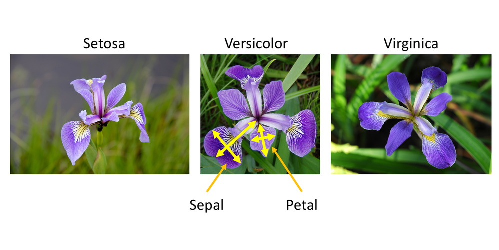
Iris flower classification is a popular dataset in machine learning projects. The dataset contains three classes of flowers: Versicolor, Virginica, Setosa and each class has 4 features like “Sepal length”, “Sepal width”, “Petal length” and “ Petal width”. The goal of the iris flower classification is to train the SVM mode and predict flowers based on their features.

As the dataset has labeled the variable, it is supervised machine learning. Supervised machine learning a is type of machine learning that are trained on well-labeled training data. Labeled data means that training data is already tagged with correct output.

In this project, I will solve the problem using neural networks: artificial neural networks (ANNs) as it is a supervised algorithm which rely on training data to learn and improve their accuracy over time. Once these learning algorithms are fine-tuned for accuracy, they are powerful tools in classification and clustering data.

How artificial neural networks work?

It is comprised of a node layers, containing an input layer, one or more hidden layers, and an output layer. Each node, or artificial neuron, connects to another and has an associated weight and threshold. If the output of any individual node is above the specified threshold value, that node is activated, sending data to the next layer of the network. Otherwise, no data is passed along to the next layer of the network.

Python Packages:

1. Numpy

2. Pandas

3. Sklearn

4. Keras

Roadmap:

1. Load the data

2. Split a dataset into training and testing datasets

3. Train the model

4. Model Evaluation

5. Testing the model

Step 1:

Import packages:

import numpy as np
import pandas as pd

from sklearn.metrics import accuracy_score
from sklearn.metrics import classification_report

from sklearn.preprocessing import LabelEncoder
from sklearn.model_selection import train_test_split
from keras.utils.np_utils import to_categorical

from keras.models import Sequential
from keras.layers import Dense
		    

First, I imported necessary packages for this project.

Numpy will be used for any computational operations.

Pandas will used to load data from various sources like local or cloud storage, database, excel file, CSV file and so on.

Accuracy_score will be used to assess accuracy.

classification_report will be used to run summary report.

keras will be used to data conversion and neural networks models.

csv_url = 'url'
columns = ['Sepal length', 'Sepal width', 'Petal length', 'Petal width', 'Class_labels']
# Load the data
df = pd.read_csv(csv_url, names=columns)
# display first 5 rows data
print(df.head())
		    

As I use the data from web server, I define the url variable and then use read_csv to read data and set the column name as per the iris data information.

Look at first five-row data in the dataset.

# Separate features and target
data = df.values
X = data[:,0:4].astype(float)
Y = data[:,4]
		    

X features a dataset including all variables used to train the model. Also, the feature data would be converted into float data format.

Y is labeled dataset including target values.

Step2: Split a dataset into training and testing datasets

l_encode = LabelEncoder()
l_encode.fit(Y)
Y = l_encode.transform(Y)
Y = to_categorical(Y)
		    

the labeled dataset must be converted to be categorical data format by lable encoder method.

X_train, X_test, y_train, y_test = train_test_split(X, Y, test_size=0.2)
		    

I split the whole dataset into two groups: training dataset and testing dataset using train_test_split by 80% verse 20%. I will use testing dataset to check the accuracy of the mode later.

Step3: Train the model

in_dim = len(data[0])-1
model = Sequential()
model.add(Dense(8, input_dim = in_dim, activation = 'relu'))
model.add(Dense(10, activation = 'relu'))
model.add(Dense(10, activation = 'relu'))
model.add(Dense(10, activation = 'relu'))
model.add(Dense(3, activation = 'softmax'))

model.compile(loss = 'categorical_crossentropy', optimizer = 'adam', metrics = ['accuracy'])
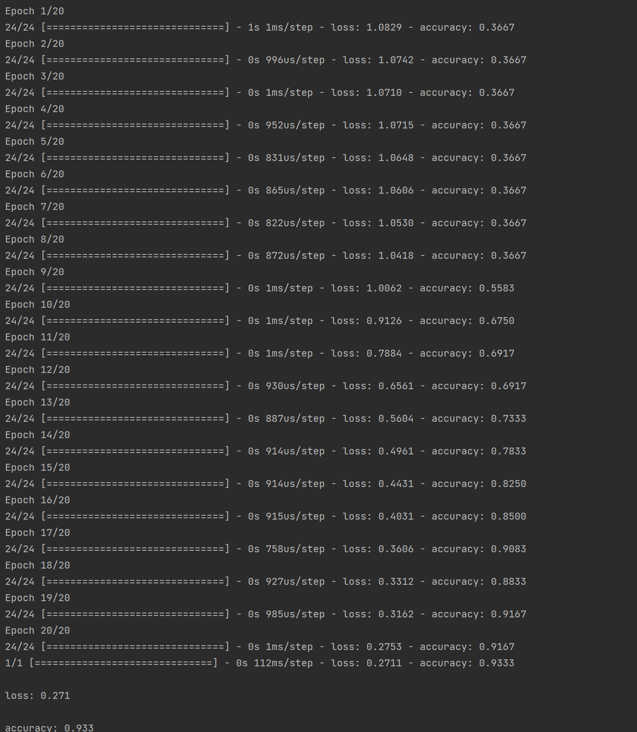
model.fit(train_x, train_y, epochs = 20, batch_size = 5)
scores = model.evaluate(test_x, test_y)

for i, m in enumerate(model.metrics_names):
    print("\n%s: %.3f"% (m, scores[i]))
		    

Build a neural network using keras with the number of features as the input dimension.

I am using ‘relu’ activation function for all layers except the output layer, where the activation function is ‘softmax’.

For multiclass classification, I have used ‘categorical crossentropy’ for loss calculation and ‘adam’ to optimize the model.

I define epochs as 20 and batch size as 5. It means the training of the neural network with the size of 5 of randomly selected training data for 20 cycles.

Step 4: Model Evaluation

Above the training results. In each epoch, I can see loss rate and Accuracy rate. It is clear that the loss rate is decreasing and Accuracy_score is increasing.

pred = model.predict(test_x)
pred_= np.argmax(pred, axis = 1)
pred_ = l_encode.inverse_transform(pred_)

true_y = l_encode.inverse_transform(np.argmax(to_categorical(test_y), axis = 1)[:,1])

for i,j in zip(pred_, true_y):
    print("Predicted: {}, True: {}".format(i, j))
    
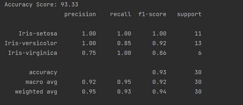
print("Accuracy Score:" ,"%.2f" % (accuracy_score(true_y, pred_)*100))
print(classification_report(true_y, pred_))
		    

I use trained the model to run prediction of test dataset and compare with labeled data to get accuracy score and summary report.

The report indicates detailed information of the prediction.

Precision defines the ration of true positives to the sum of true positive and false positive.

Recall defines the ratio of true positive to sum of true positive and false negative.

F1-score is the mean of precision and recall results.

Support is the number of actual occurrences of the class in the testing dataset.

Accuracy is the average of f1-scores.

The output accuracy result is above 93%.

Step 5: Testing the model

#Testing
X_new = np.array([[3, 2, 1, 0.2], [4.9, 2.2, 3.8, 1.1], [5.3, 2.5, 4.6, 1.9]]).astype(float)
pred_new = model.predict(X_new)
pred_new_= np.argmax(pred_new, axis = 1)
pred_new_ = l_encode.inverse_transform(pred_new_)

print("Prediction of Species: {}".format(pred_new_))
		    

I just randomly generated values based on the average plot to see if the model work correctly.

It looks like the model predicts correctly because the outputs meet expectations that setosa is shortest and virginica is longest and versicolor is in the middle.