Multi-Variant Classification

Project information

Category: Logistic Regression Model, Classification
Source Data: Download

Project Details

Description

Parkinson's disease is a brain disorder that causes unintended or uncontrollable movements, such as shaking, stiffness, and difficulty with balance and coordination. Symptoms usually begin gradually and worsen over time. As the disease progresses, people may have difficulty walking and talking. The dataset contains two classes of status: 1 meaning yes and 0 meaning no and each class has 24 features.

Data Description:

name - ASCII subject name and recording number

MDVP:Fo(Hz) - Average vocal fundamental frequency

MDVP:Fhi(Hz) - Maximum vocal fundamental frequency

MDVP:Flo(Hz) - Minimum vocal fundamental frequency

MDVP:Jitter(%),MDVP:Jitter(Abs),MDVP:RAP,MDVP:PPQ,Jitter:DDP - Several

measures of variation in fundamental frequency

MDVP:Shimmer,MDVP:Shimmer(dB),Shimmer:APQ3,Shimmer:APQ5,MDVP:APQ,Shimmer:DDA - Several measures of variation in amplitude

NHR,HNR - Two measures of ratio of noise to tonal components in the voice

status - Health status of the subject (one) - Parkinson's, (zero) - healthy

RPDE,D2 - Two nonlinear dynamical complexity measures

DFA - Signal fractal scaling exponent

spread1,spread2,PPE - Three nonlinear measures of fundamental frequency variation

The goal of the Parkinson’s disease is to train the random forest model, analyze importance of variables, tuning the accuracy of model, predict status based on their features.

As the dataset have labeled the variable, it is supervised machine learning. Supervised machine learning are types of machine learning that are trained on well-labeled training data. Labeled data means that training data is already tagged with correct output.

In this project, I will solve the problem using the algorithm: logistic regression as it is a supervised machine learning algorithm which analyzes data for classification. Also, logistic regression is one of the most robust classification methods.

Based on the tasks performed and the nature of the output, you can classify machine learning models into three types:

Regression: where the output variable to be predicted is a continuous variable.

Classification: where the output variable to be predicted is a categorical variable.

Clustering: where there is no pre-defined notion of a label allocated to the groups/clusters formed.

Types of Logistic Regression:

Binary (true/false, yes/no)

Multi-class (sheep, cats, dogs)

Ordinal (Job satisfaction level — dissatisfied, satisfied, highly satisfied)

Methodology

Logistic regression is a linear classifier, so you’ll use a linear function 𝑓(𝐱) = 𝑏₀ + 𝑏₁𝑥₁ + ⋯ + 𝑏ᵣ𝑥ᵣ, also called the logit. The variables 𝑏₀, 𝑏₁, …, 𝑏ᵣ are the estimators of the regression coefficients, which are also called the predicted weights or just coefficients.

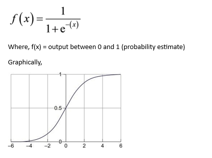
The logistic regression function 𝑝(𝐱) is the sigmoid function of 𝑓(𝐱): 𝑝(𝐱) = 1 / (1 + exp(−𝑓(𝐱)). As such, it’s often close to either 0 or 1. The function 𝑝(𝐱) is often interpreted as the predicted probability that the output for a given 𝐱 is equal to 1. Therefore, 1 − 𝑝(𝑥) is the probability that the output is 0.

Python Packages:

1. Matplotlib

2. Seaborn

3. Pandas

4. Scikit-learn

5. Numpy

Roadmap:

1. Load the data

2. Analyze and visualize the dataset

3. Split a dataset into training and testing datasets

4. Train the model

5. Model Evaluation

6. Testing the model

7. Improving performance

Step 1:

Import packages:

#import libaries
import pandas as pd
import seaborn as sns
import numpy as np
import matplotlib.pyplot as plt
from sklearn.model_selection import train_test_split
from sklearn.metrics import accuracy_score
from sklearn.metrics import classification_report
from sklearn.linear_model import LogisticRegression

First, I imported necessary packages for this project.

Pandas will used to load data from various sources like local or cloud storage, database, excel file, CSV file and so on.

Matplotlib and seaboarn will be used for data visualization.

Numpy will be used to data transfer and list manipulation.

Sklearn will be used for data split, accuracy report and modeling.

#Read the data
url=r'url'
df=pd.read_csv(url)
print(df.head())

As I use the data from web server, I define the url variable and then use read_csv to read data and set the column name as per the iris data information.

Look at first five-row data in the dataset.

Step2: Analyze and visualize the dataset

# display base statistical analysis regarding the data
print(df.describe())

From this data description, I can see all the data descriptions on the data, like mean in different measurements, min and max values and 25%, 50% and 75% distribution values.

Let’s visualize the dataset.

Seaborn pair plot method helps visualize the whole dataset.

By looking the visualization, it is very clear that those whose status is yes have all values higher than those whose status is no.

# Separate features and target
X=df.loc[:,df.columns!='status'].values[:,1:]
Y=df.loc[:,'status'].values
feature=df.drop(['name','status'], axis=1)
feature_list=list(feature.columns)
Y = data[:,4]

X features a dataset including all variables used to train the model.

Y is labeled dataset including target values.

Step3: Split a dataset into training and testing datasets

X_train, X_test, y_train, y_test = train_test_split(X, Y, test_size=0.20, random_state=42)

I split the whole dataset into two groups: training dataset and testing dataset using train_test_split by 80% verse 20%. I will use the testing dataset to check the accuracy of the mode later.

Step4: Train the model

LR=LogisticRegression(solver='liblinear', max_iter=3000,  C=10, random_state=0)
LR.fit(X_train,y_train)

initialize logistic regression class from scikit-learn package to LR variable.

Set the solver is liblinear which is default, max_iter to 3000, and C=10

solver is a string ('liblinear' by default) that decides what solver to use for fitting the model. Other options are 'newton-cg', 'lbfgs', 'sag', and 'saga'.
max_iter is an integer (100 by default) that defines the maximum number of iterations by the solver during model fitting.
C is a positive floating-point number (1.0 by default) that defines the relative strength of regularization. Smaller values indicate stronger regularization.
random_state is an integer, an instance of numpy.RandomState, or None (default) that defines what pseudo-random number generator to use.

I feed training dataset and labeled dataset into the algorithm using fit() method.

Step 5: Model Evaluation

pred=LR.predict(X_test)
print('First Run Performance:'+str(accuracy_score(y_test,pred)*100))

I predict the classes from testing dataset using my trained model.

Check the accuracy score of the predicted results.

Accuracy_score takes true values and predicted values and return percentage of accuracy.

I also show the detailed classification repot based the testing dataset.

print(classification_report(y_test, pred))

The report indicates detailed information of the prediction.

Precision defines the ration of true positives to the sum of true positive and false positive.

Recall defines the ratio of true positive to sum of true positive and false negative.

F1-score is the mean of precision and recall results.

Support is the number of actual occurrences of the class in the testing dataset.

Accuracy is the average of f1-scores.

print("Interception:"+str(LR.intercept_))
print("Conefficients:"+str(LR.coef_))
print("Training Accuracy:"+str(LR.score(X_train,y_train)))

As you can see, 𝑏₀ is given inside a one-dimensional array, while 𝑏₁ is inside a two-dimensional array. You use the attributes .intercept_ and .coef_ to get these results.

Step 6: Testing the Model

#Testing the model
X_new = np.array([[180.19800,201.24900,175.45600,0.00284,0.00002,0.00153,0.00166,0.00459,0.01444,0.13100,0.00726,0.00885,0.01190,0.02177,0.00231,26.73800,0.403884,0.766209,-6.452058,0.212294,2.269398,0.141929],
                  [241.40400,248.83400,232.48300,0.00281,0.00001,0.00157,0.00173,0.00470,0.01760,0.15400,0.01006,0.01038,0.01251,0.03017,0.00675,23.14500,0.457702,0.634267,-6.793547,0.158266,2.256699,0.117399],
                  [242.85200,255.03400,227.91100,0.00225,0.000009,0.00117,0.00139,0.00350,0.01494,0.13400,0.00847,0.00879,0.01014,0.02542,0.00476,25.03200,0.431285,0.638928,-6.995820,0.102083,2.365800,0.102706]])
pred_new = LR.predict(X_new)
# expected results:1,0,0
print("Prediction of Parkinson's Status : {}".format(pred_new))

I just randomly generated values based on the average plot to see if the model work correctly.