Group Data Analysis

Project information

Category: Modeling, Regression
Source Data: statsmodels Package

Project Details

Data Description

Growth curves of pigs data contains weight of slaughter pigs measured weekly for 12 weeks. Data also contains the startweight (i.e. the weight at week 1). The treatments are 3 different levels of Evit = vitamin E (dose: 0, 100, 200 mg dl-alpha-tocopheryl acetat /kg feed) in combination with 3 different levels of Cu=copper (dose: 0, 35, 175 mg/kg feed) in the feed. The cumulated feed intake is also recorded. The pigs are littermates.

Weight: Weight in Kg

Feed: Cumulated feed intake in Kg

Time: Time (in weeks) in the experiment

Pig: Factor; id of each pig

Evit: Factor; vitamin E dose; see Data Description

Cu: Factor, copper dose; see Data Description

Start: Start weight in experiment, i.e. weight at week 1

Litter: Factor, id of litter of each pig

The goal of the Growth curves of pigs is to train mixed effect regression model, analyze the weight of pig, tuning the accuracy of model, predict weight based on their features.As the dataset has labeled the variable, it is supervised machine learning. Supervised machine learning is a type of machine learning that is trained on well-labeled training data. Labeled data means that training data is already tagged with correct output. In this project, I will solve the problem using the algorithm: mixed effect regression as data is longitudinal. Also, mixed effect regression is one of the most robust regression methods.

What is mixed effect regression?

Mixed effects regression is an extension of the general linear model (GLM) that considers the hierarchical structure of the data. Mixed effect models are also known as multilevel models, hierarchical models, mixed models (or specifically linear mixed models (LMM)) and are appropriate for many types of data such as clustered data, repeated-measures data, longitudinal data, as well as combinations of those three. Since mixed effects regression is an extension of the general linear model, let's recall that the general linear regression equation looks like:

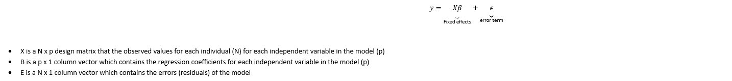
Fixed factors are the independent variables that are of interest to the study, e.g. treatment category, sex or gender, categorical variable, etc.

Random factors are the classification variables that the unit of anlaysis is grouped under, i.e. these are typically the variables that define level 2, level 3, or level n. These factors can also be thought of as a population where the unit measures were randomly sampled from, i.e. (using the school example from above) the school (level 2) had a random sample of students (level 1) scores selected to be used in the study.

Python Packages:

1. Matplotlib

2. Seaborn

3. researchpy

4. statsmodels

5. scipy

Roadmap:

1. Load the data

2. Analyze and visualize the dataset

3. Train the model

4. Assumption Check

5. Testing the model

Step 1:

Import packages:

#import libaries
import statsmodels.api as sm
import statsmodels.formula.api as smf
import researchpy as rp
import matplotlib.pyplot as plt
import scipy.stats as stats
import seaborn as sns
from statsmodels.stats.diagnostic import het_white
import warnings

First, I imported necessary packages for this project.

df = sm.datasets.get_rdataset('dietox', 'geepack').data
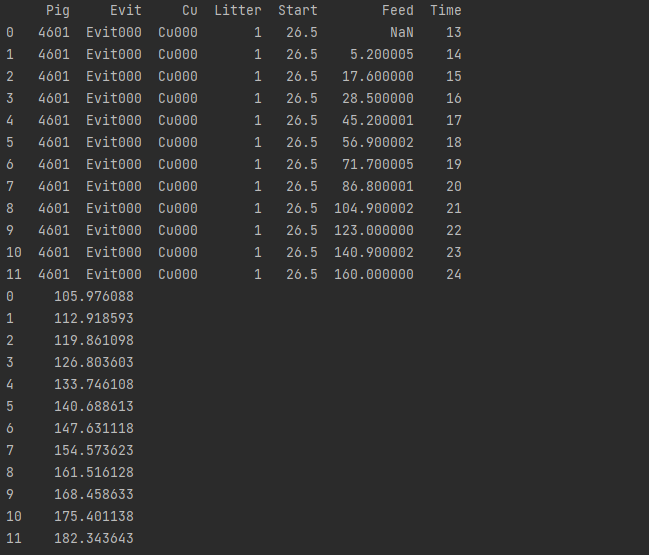
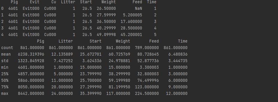
print(df.head())
print(df.describe())

Load data from statsmodels package.

Look at the first five-row data in the dataset.

Look at statistics on variables in the dataset.

From this data description, I can see all the data descriptions on the data, like mean in different measurements, min and max values and 25%, 50% and 75% distribution values.

Step2: Analyze and visualize the dataset

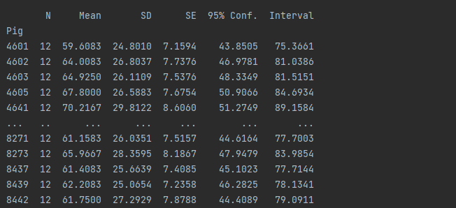
print(rp.summary_cont(df.groupby(['Pig'])['Weight']))

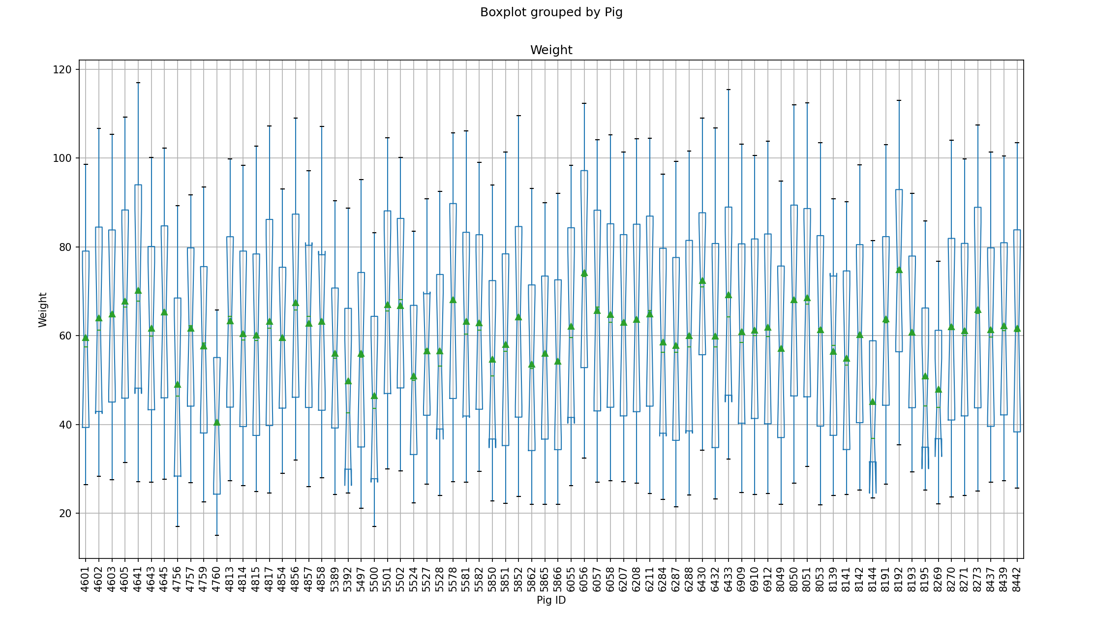
Take a look at the weight of the pig based on individual group.

Looking at data, I have a general idea of the growth range for individual pig. Range should be mean+/- SD.

boxplot = df.boxplot(["Weight"], by = ["Pig"],
                     figsize = (16, 9),
                     showmeans = True,
                     notch = True)

boxplot.set_xlabel("Pig ID")
boxplot.set_ylabel("Weight")
plt.xticks(rotation='vertical')
plt.show()

Visualize the distribution of weight by pig group. For this, the built-in Pandas boxplot method will be used. Seaborn and Matplotlib are other great graphing libraries for Python.

The line that goes across the box is the median value and the triangle is the mean value. The notched boxes in this case show the confidence interval of the median. Any symbol that is above/below the whisker of the box is being indicated as a potential outlier.

The distribution and variables of weights look fairly similar, but the variance looks different across start weights.

Step 3: Train the model

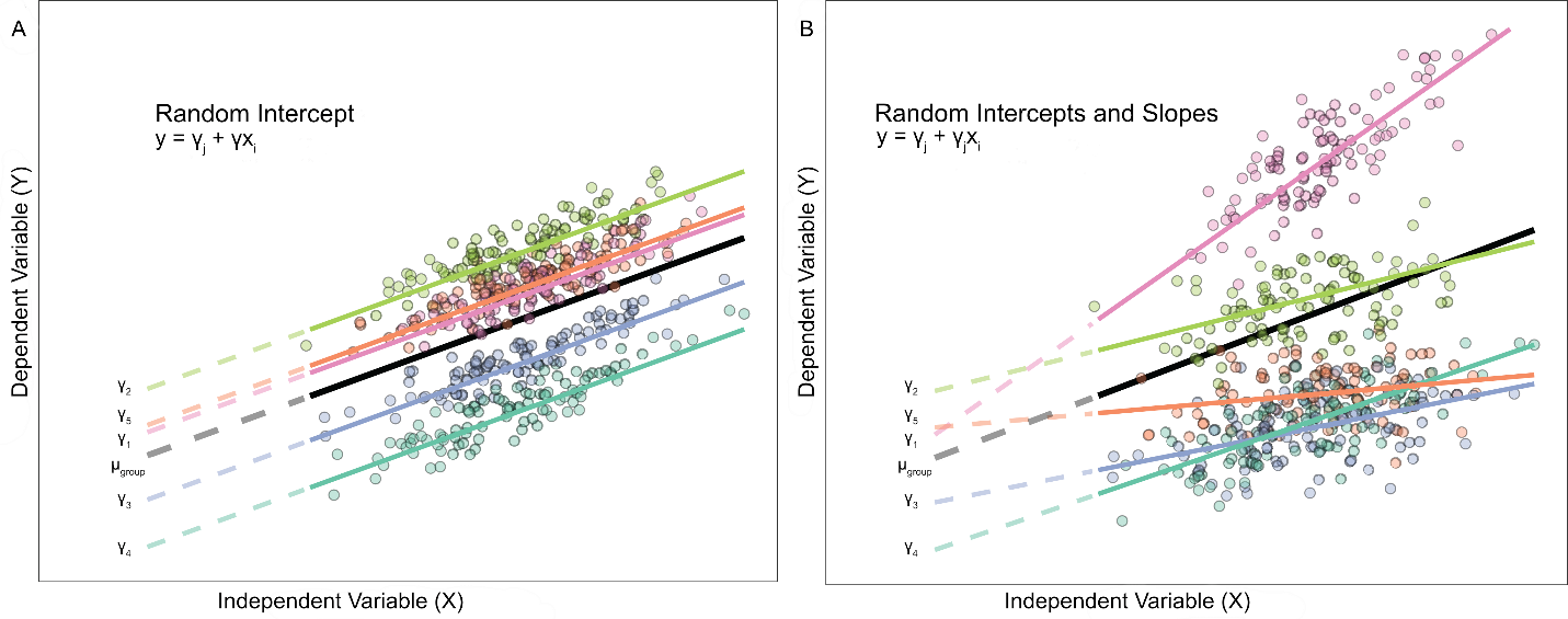
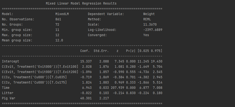
# Random intercepts
model1 = smf.mixedlm("Weight ~ Time+C(Evit,Treatment('Evit000'))+C(Cu,Treatment('Cu000'))+Litter",df,groups= "Pig").fit()
print("Random intercepts")
print(model1.summary())

To fit a random intercept model, this type of model allows for different clusters to have different intercepts.

The pig var is the random effects of the cluster variable. It models the variation that is present between the pigs. I can convert the variance to standard deviation by taking the square root. This means the on average the pig weight can vary about 6.35 kgs.

The Evit and Cu are non-significant, so they will be removed from the model and re-run.

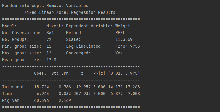
# Random intercepts removed variables
model11 = smf.mixedlm("Weight ~ Time",df,groups= "Pig").fit()
print("Random intercepts Removed Variables")
print(model11.summary())

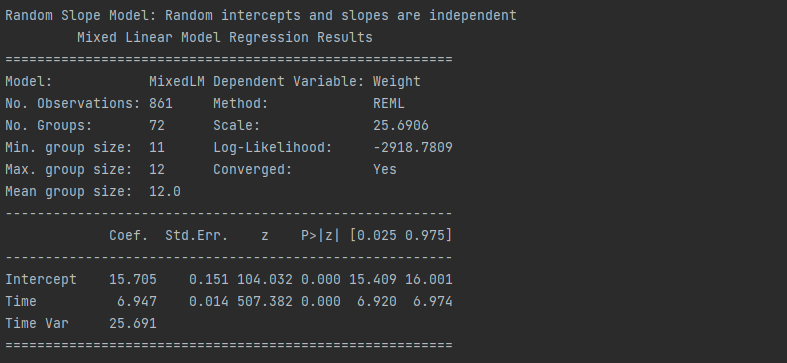
Intraclass correlation coefficient (ICC) is another useful statistic which measures the similarity of the responses within a random effect. In the current model with 1 cluster variable, this would be the similarity in weights in the pig. The ICC can range between 0 to 1 where 1 indicates perfect relationship within the clusters. To calculate the ICC, it takes the variance of the cluster variable (40.394) and divides it by the unexplained variance of the model (11.3669). The result is 3.55 which indicates that there is a moderate level of correlation between weights within a pig.

# Random Slope Model: Random intercepts and slopes are independent
model2 = smf.mixedlm("Weight ~ Time",df,groups= "Pig", vc_formula = {"Time" : "0 + C(Time)"}).fit()
print("Random Slope Model: Random intercepts and slopes are independent")
print(model2.summary())

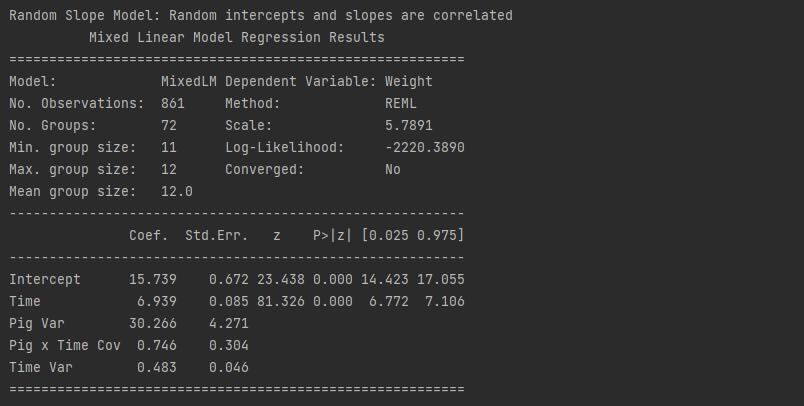
Using the same data, a random slop model will be fit where the random intercepts and slops are independent. In this model, a slope will be time.

The estimated variance for random time slopes is 25.691 which is a standard deviation of 5.07. It indicates that from cluster to cluster, i.e between pig, the time slope fluctuates by +/- 5.07.

# Random Slope Model: Random intercepts and slopes are correlated
model3 = smf.mixedlm("Weight ~ Time",df,groups= "Pig", re_formula="Time").fit()
print("Random Slope Model: Random intercepts and slopes are correlated")
print(model3.summary())

Using the same data, a random slope model will be fit where the random intercept and slopes are correlated. In this model, a random slope will be allowed for the time.

Including random intercepts and random slopes is useful to calculate the estimated correlation between the random intercepts and random slopes. This is calculated by taking the co-variance of the random intercept (clustering variable) and random slope (random slope variable) and dividing it by the product of the variance of the random intercept and the variance of the random slope variable.

0.746/sqrt(30.266*0.483)=0.195

It indicates that the pigs with higher weight tend to have times that are of higher weight.

Step 4: assumption check

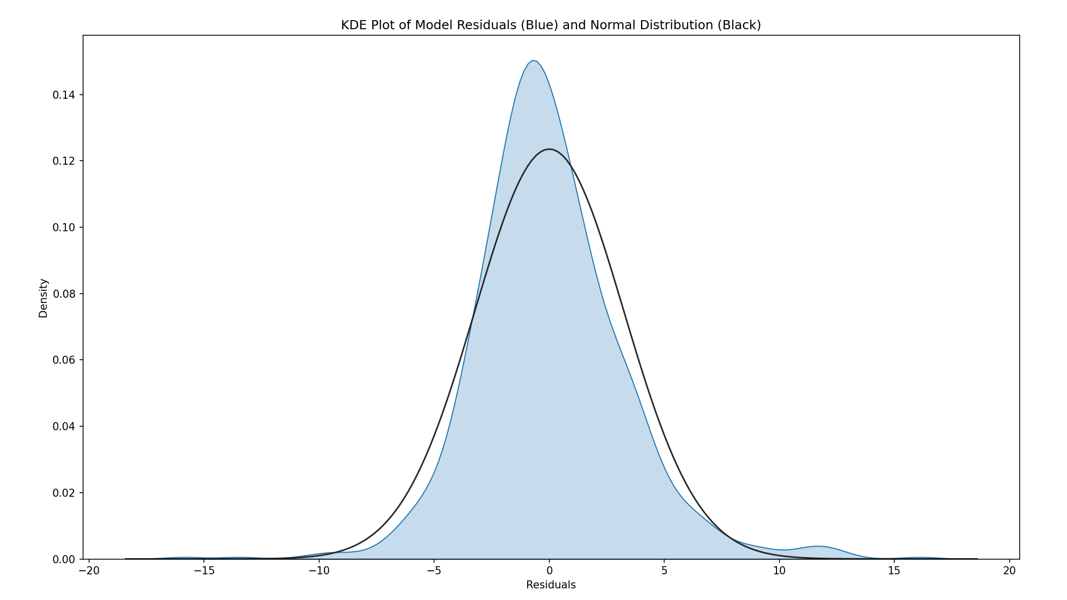
Linear mixed effect models have the same assumption as the traditional standard linear regression model. For the model diagnostics, I will use the random intercept with clustering variable being pig.

One can check for normality of the residuals graphically, a formal statistical test, or a combination of the two. If the overall sample is large one should use both since as the sample size increases so does the power of the tests, meaning that the larger the sample size the smaller of a difference the formal statistical test will detect and a significant p-value will be provided.

#NORMALITY
fig = plt.figure(figsize = (16, 9))
ax = sns.distplot(model3.resid, hist = False, kde_kws = {"shade" : True, "lw": 1}, fit = stats.norm)
ax.set_title("KDE Plot of Model Residuals (Blue) and Normal Distribution (Black)")
ax.set_xlabel("Residuals")
plt.show()

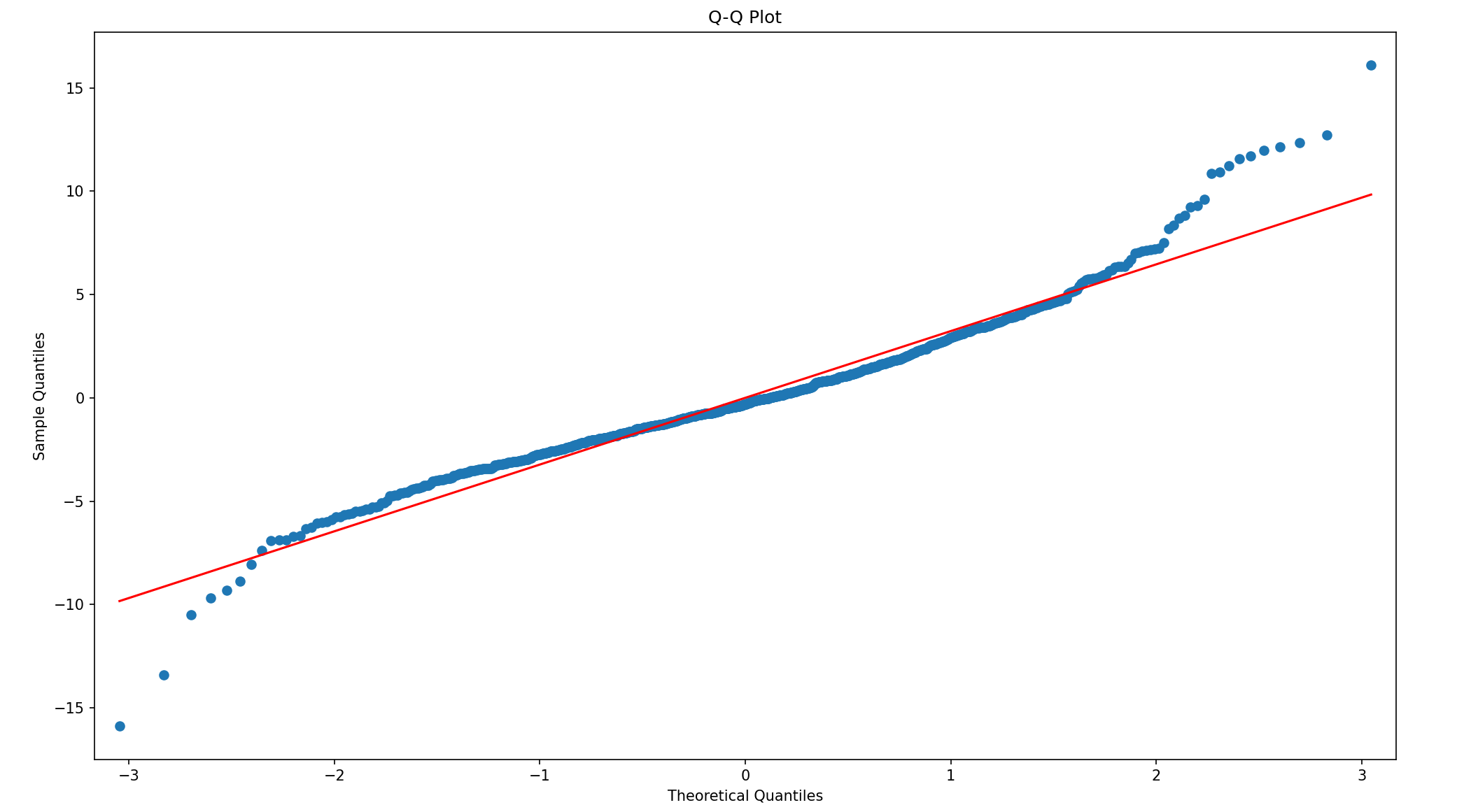
Visualize the residuals with a kernal density estimate plot.

## Q-Q PLot
fig = plt.figure(figsize = (16, 9))
ax = fig.add_subplot(111)
sm.qqplot(model11.resid, dist = stats.norm, line = 's', ax = ax)
ax.set_title("Q-Q Plot")
plt.show()

There is some deviation from normality, but it does not look concerning. There are a couple of outliers which are evident in both plots. How to address the outlier is up to the researcher.

# Shapir-Wilk test of normality
labels = ["Statistic", "p-value"]
norm_res = stats.shapiro(model11.resid)
for key, val in dict(zip(labels, norm_res)).items():
    print(key, val)

The test is significant which indicates that the assumption of normality for the residuals is violated. This would suggest that the model could be adjusted to meet this assumption. Common techniques include transform variables, remove outliers, use a non-parametric approach, or rely on the central limit theorem.

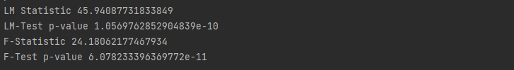
# homoskedasticity 
fig = plt.figure(figsize = (16, 9))
ax = sns.scatterplot(y = model11.resid, x = model11.fittedvalues)
ax.set_title("RVF Plot")
ax.set_xlabel("Fitted Values")
ax.set_ylabel("Residuals")
plt.show()

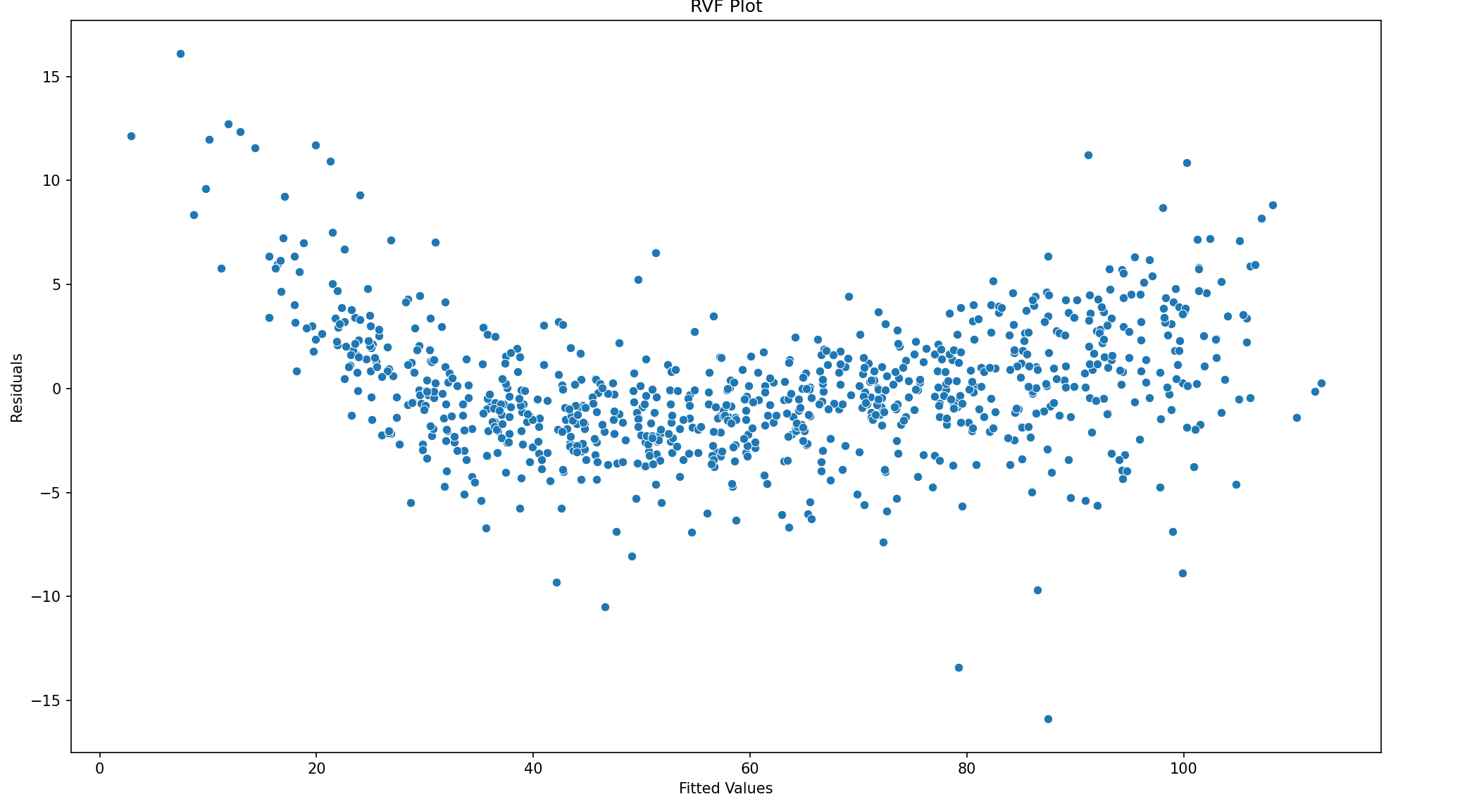
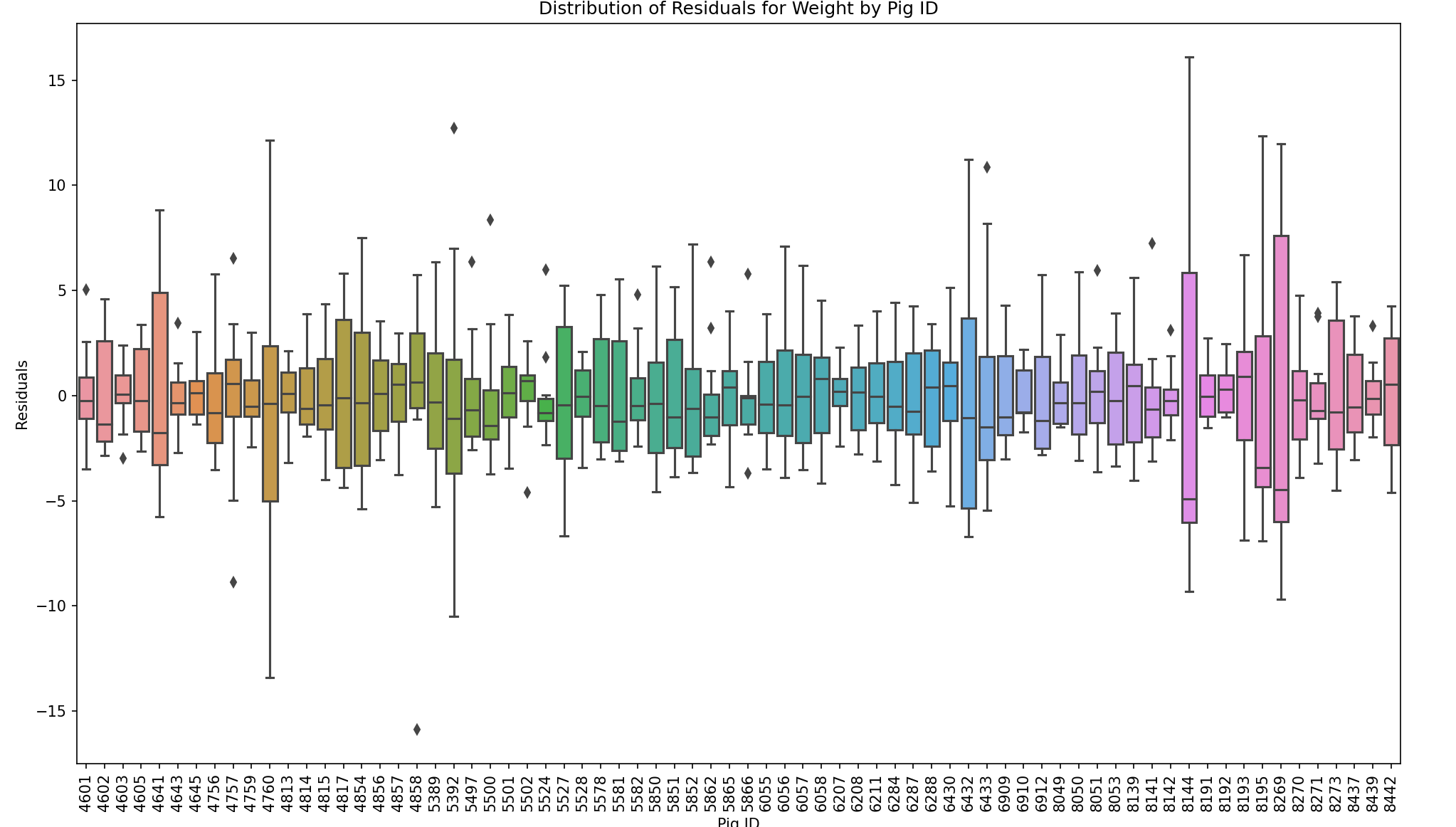
I can check for homoskedasticity of variance visually, with a formal test, or both.

fig = plt.figure(figsize = (16, 9))
ax = sns.boxplot(x = model11.model.groups, y = model11.resid)
ax.set_title("Distribution of Residuals for Weight by Pig ID")
ax.set_ylabel("Residuals")
ax.set_xlabel("Pig ID")
plt.xticks(rotation='vertical')
plt.show()

Test this assumption with the White’s Lagrange Multiplier Test for Heteroscedasticity.

Based on the visual tests, it appears that there isn't much concern about violating the assumption of homoskedasticity of the variance; however, the formal testing indicates this assumption is violated.

Step 5: test the model

# Testing the model
test_file_path=r'C:\Users\shang\Desktop\ML\data\pig_test.csv'
test=pd.read_csv(test_file_path)
print(test)
pred=model11.predict(exog=test)
print(pred)

I create a test data file for one pig.

Read the test data file.

Displayed data.

Feed data to model.

Predict the weights based on time.

Since the last record for the pig: 4601 shows the weight as 98.59998, the expected weight should be greater than the last weight and increased. The predicted values meet my expectations.