Convolution Neural Network

Project Details

Data Description

In this project, I used use CIFAR-10 dataset which consists of 50000 32*32 color images in 10 classes with 5000 images per class.

Here are 10 classes:

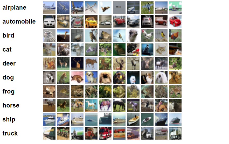
As the dataset has labeled the variable, it is supervised machine learning. Supervised machine learning a is type of machine learning that is trained on well-labeled training data. Labeled data means that training data is already tagged with correct output.

In this project, I will solve the problem using neural networks: convolutional neural networks (CNN) as it is a supervised algorithm which rely on training data to learn and improve their accuracy over time.

What is CNN?

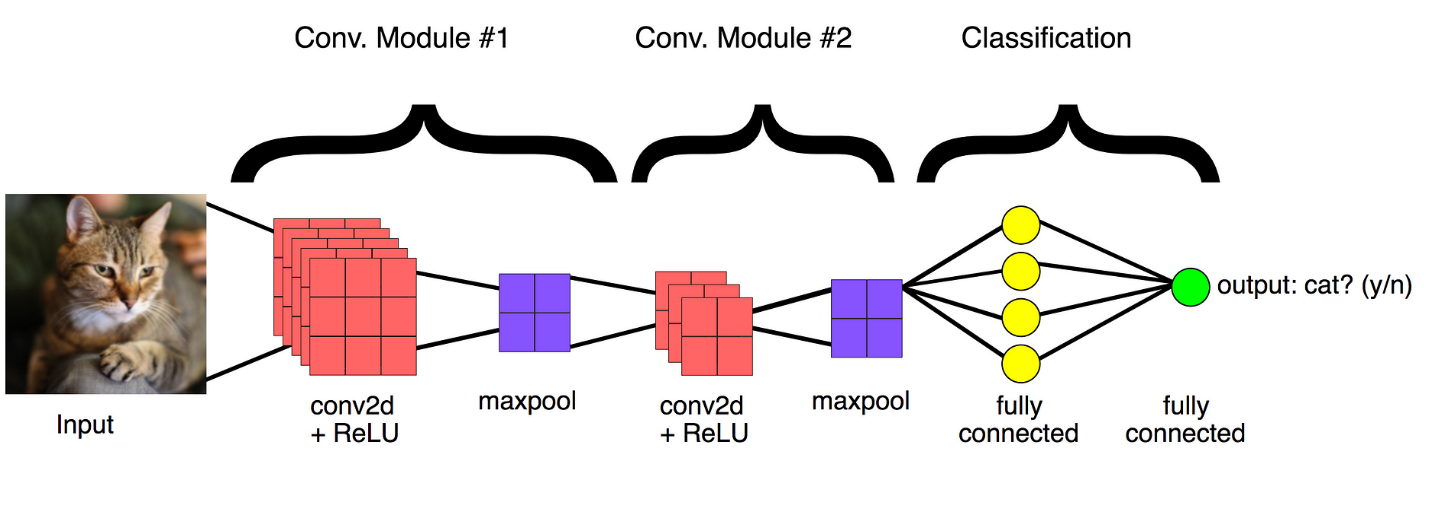
CNN is a combination of Convolutional Layers and Neural Network. Convolution is nothing but a filter which is applied on an image to extract features from it. We will use such different convolutions to extract different features like edges highlighted patterns from the image.

Python Packages:

1. Pandas
2. Keras
3. Numpy
4. matplotlib

Roadmap:

1. Load the data

2. Split a dataset into training and testing datasets

3. Train the model

4. Model Evaluation

5. Generate Output

Step 1:

Import packages:

from keras.models import Sequential
from keras.preprocessing.image import ImageDataGenerator
from keras.layers import Dense, Activation, Flatten, Dropout, BatchNormalization
from keras.layers import Conv2D, MaxPooling2D
import pandas as pd
import numpy as np
from keras.models import load_model
import matplotlib.pyplot as plt
from keras.callbacks import EarlyStopping, ReduceLROnPlateau
		    

First, I imported necessary packages for this project.

Pandas will used to load data from various sources like local or cloud storage, database, excel file, CSV file and so on.

Numpy will be used for any computational operations.

keras will be used to data conversion and neural networks models.

Matplotlib will be used to plot a chart for model evaluation.

def append_ext(fn):
    return fn + ".png"
		    

As training data is a png file format, this function will append extension file automatically.

train_label_path = r'C:\Users\shang\Desktop\ML\data\image classification\trainLabels.csv'
sub_file_path = r'C:\Users\shang\Desktop\ML\data\image classification\sampleSubmission.csv'
train_folder_path=r'C:\Users\shang\Desktop\ML\data\image classification\train'
test_folder_path=r'C:\Users\shang\Desktop\ML\data\image classification\test'

traindf = pd.read_csv(train_label_path, dtype=str)
testdf = pd.read_csv(sub_file_path, dtype=str)

traindf["id"] = traindf["id"].apply(append_ext)
testdf["id"] = testdf["id"].apply(append_ext)
		    

Defined the path variable and then use read_csv to read data and automatically add file extension name.

Step2: Split a dataset into training and testing datasets

datagen = ImageDataGenerator(rescale=1. / 255., validation_split=0.25)
		    

Defined scale ratio for resizing the image and split ratio %75:training versus %25:validation for training a model.

Step3: Train the model

train_generator=datagen.flow_from_dataframe(
                                            dataframe=traindf,
                                            directory=train_folder_path,
                                            x_col="id",
                                            y_col="label",
                                            subset="training",
                                            batch_size=32,
                                            seed=42,
                                            shuffle=True,
                                            class_mode="categorical",
                                            target_size=(32,32))
		    

Defined the flow from dataframe which was used for training data.

valid_generator=datagen.flow_from_dataframe(
                                            dataframe=traindf,
                                            directory=train_folder_path,
                                            x_col="id",
                                            y_col="label",
                                            subset="validation",
                                            batch_size=32,
                                            seed=42,
                                            shuffle=True,
                                            class_mode="categorical",
                                            target_size=(32,32))
		    

Defined the flow from dataframe which was used for validation data.

test_datagen=ImageDataGenerator(rescale=1./255.)
		    

Defined scale ratio for resizing the image for testing.

test_generator=test_datagen.flow_from_dataframe(
                                                dataframe=testdf,
                                                directory=test_folder_path,
                                                x_col="id",
                                                y_col=None,
                                                batch_size=32,
                                                seed=42,
                                                shuffle=False,
                                                class_mode=None,
                                                target_size=(32,32))
		    

Defined the flow from dataframe which was used for testing dataset as I do not know the result. I set y_col as none.

earlystop = EarlyStopping(patience=10)
learning_rate_reduction = ReduceLROnPlateau(monitor='val_accuracy', patience=2, verbose=1, factor=0.5, min_lr=0.00001)
callbacks = [earlystop, learning_rate_reduction]
		    

EarlyStopping refers to stop training when a monitored metric has stopped improving.

ReduceLROnPlateau refers to reduce learning rate when a metric has stopped improving. Models often benefit from reducing the learning rate by a factor of 2-10 once learning stagnates. This callback monitors a quantity and if no improvement is seen for a 'patience' number of epochs, the learning rate is reduced.

model = Sequential()
model.add(Conv2D(32, (3, 3), activation='relu', padding='same',input_shape=(32,32,3)))
model.add(BatchNormalization())
model.add(Conv2D(32, (3, 3), activation='relu'))
model.add(MaxPooling2D(pool_size=(2, 2)))
model.add(Dropout(0.25))
model.add(Conv2D(64, (3, 3), activation='relu',padding='same'))
model.add(Conv2D(64, (3, 3), activation='relu'))
model.add(MaxPooling2D(pool_size=(2, 2)))
model.add(Dropout(0.25))
model.add(Flatten())
model.add(Dense(512, activation='relu'))
model.add(BatchNormalization())
model.add(Dropout(0.5))
model.add(Dense(10, activation='softmax'))
model.compile(loss='categorical_crossentropy', optimizer='adam', metrics=['accuracy'])
print(model.summary())
		    

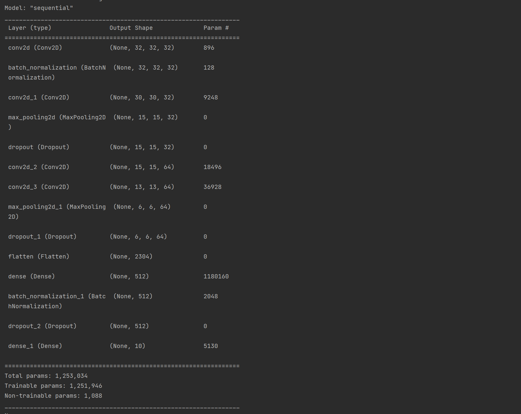
For Conv2D, I define 32 filters and each filter has 3*3 size and use relu activation. It starts performing element-wise multiplication starting from the top left corner of the image. Element-wise multiplication means multiplying elements with same index. These computed values are summed up to obtain a pixel value and it is stored in the new matrix which will be used for further processing.

For BatchNormalization, it is a technique for training very deep neural networks that standardizes the input to layer for each mini-batch. It has the effect of stabilizing the learning process and dramatically reducing the number of training epochs required to train deep networks.

For MaxPooling2D, It selects maximum values from the matrix of specified size( default 2*2). This method is helpful to extract features with high importance or which are high-lighted in the image.

For Dropout, it randomly select and drop off some of the layers neurons, by which is achieved an ensemble effect (due to random select- each time different neurons are deactivated, each time different network predicting). It helps prevent from overfitting.

For Flatten, it converts multi-dimensional matrix to single dimensional matrix.

For Dense, it is simple layer of neurons in which each neuron receives input from all the neurons of previous layer, called dense. Dense layer is used to classify image based on output from convolutional layers.

Output layer has 10 neurons with softmax activation function. Softmax activation function is used when we have 2 or more classes. If we have total 10 classes, then the number of neurons in the output layer will be 10. Each neuron represents one class.

So, all 10 neurons will return probabilities of the input image for the respective class. Class with the highest probability will be considered as output for the image.

Summary() displays the architecture of the model.

Parameters(params) are the weights and biases that will be used for computation in all neurons of the CNN. When we train any model on some number of images, it will determine some specific values for all parameters (weights and biases), which are used to process the image and predict the output of the image.

STEP_SIZE_TRAIN=train_generator.n//train_generator.batch_size
STEP_SIZE_VALID=valid_generator.n//valid_generator.batch_size
STEP_SIZE_TEST=test_generator.n//test_generator.batch_size
his=model.fit_generator(generator=train_generator,
                    steps_per_epoch=STEP_SIZE_TRAIN,
                    validation_data=valid_generator,
                    validation_steps=STEP_SIZE_VALID,
                    epochs=10,  callbacks=callbacks
		    

Feed training data and validation data into model and train the model.

How to calculate steps:

Split the training set into many batches. When running the algorithm, it requires one epoch to analyze the full training set. An epoch is composed of many iterations (or batches).

Iterations: the number of batches needed to complete one Epoch.

Batch Size: The number of training samples used in one iteration.

Epoch: one full cycle through the training dataset. A cycle is composed of many iterations.

Number of Steps per Epoch = (Total Number of Training Samples) / (Batch Size)

Example: there are a total of 2000 images and batch size is 10. So, the number of steps per epoch is 2000/10=200 steps.

Loss refers to the loss value over the training data after each epoch. This is what the optimization process is trying to minimize with training so, the lower, the better.

Accuracy refers to the ratio between correct predictions and the total number of predictions in the training data. The higher, the better.

Val_loss refers to the loss value over the validation data after each epoch.

Val_accuracy refers to the ratio between correct predictions and the total number of predictions in the validation data.

Lr refers to Learning rate indicates how big or small the changes in weights are after each optimisation step.

Step 4: Model Evaluation

model.save("model_cifar_10epoch.h5")

acc=model.evaluate_generator(generator=valid_generator,steps=STEP_SIZE_VALID)
print(acc*100)
		    

Save the trained model for later use.

Evaluate accuracy using validation data.

#Plot the training and valiation loss
fig, axs = plt.subplots(2)
fig.suptitle('Model Evaluation')
#Assign the first subplot to graph training loss and validation loss
axs[0].plot(his.history['loss'],color='b',label='Training Loss')
axs[0].plot(his.history['val_loss'],color='r',label='Validation Loss')
axs[0].set_title('Loss', fontfamily='serif', loc='left', fontsize='medium')
axs[0].legend(loc='upper center')
#Next lets plot the training accuracy and validation accuracy
axs[1].plot(his.history['accuracy'],color='b',label='Training  Accuracy')
axs[1].plot(his.history['val_accuracy'],color='r',label='Validation Accuracy')
axs[1].set_title('Accuracy', fontfamily='serif', loc='left', fontsize='medium')
axs[1].legend(loc='upper center')
plt.show()
		    

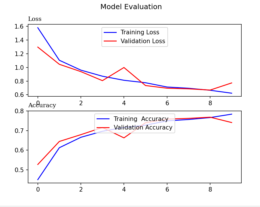
It is evident that the model starts overfitting at around 8 epochs where I find that the validation accuracy starts dropping, however the training accuracy keeps increasing. The validation accuracy at this point is around 75%. This could probably be because the images are only 32 *32 pixels.

Step 5: Generate Output

maps = {
    0: 'airplane',
    1: 'automobile',
    2: 'bird',
    3: 'cat',
    4: 'deer',
    5: 'dog',
    6: 'frog',
    7: 'horse',
    8: 'ship',
    9: 'truck'
}
test_generator.reset()
pred=model.predict(test_generator,steps=STEP_SIZE_TEST,verbose=1)
predicted_class_indices = np.argmax(pred, axis=1)
predictions = [maps[k] for k in predicted_class_indices]

filenames = test_generator.filenames
results = pd.DataFrame({"Filename": filenames,
                        "Predictions": predictions})
results.to_csv("model_cifar_10epoch.csv", index=False)
		    

The map dictionary will be used to map numeric values to content.

Reset the test generator.

Run prediction to use test data to predict results.

As the output will be a list which consists of probability of each class the pickup the max value which will be predicted result.

Combined test image filenames and predicted results together and generate output file in csv format.

In conclusion, the model is overfitting because of low resolution which are 32 *32 pixels. To improve accuracy, probably, I need to use well-trained models like Inception, VGG16, VGG19, mobilenet, etc which are created by some researchers after training them on millions of images to classify images.